Robotics · Control Systems · Simulation

ABB IRB120 Robot Arm
Modelling & Simulation

A complete mathematical model and dynamic simulation of the ABB IRB120 6-DOF industrial robot arm — from DH parameter derivation through Lagrangian dynamics, trajectory generation, and Simulink-based SimMechanics simulation.

Type
Bachelor Thesis
Institution
Istanbul Aydın University
Advisor
Prof. Gökhan Erdemir
Date
June 2014
Status
Completed
Matlab Simulink ABB IRB120 6-DOF Denavit–Hartenberg Forward Kinematics Inverse Kinematics Lagrangian Dynamics Trajectory Planning SimMechanics
01 — Abstract

Project overview

This project develops a full mathematical model and dynamic simulation of the ABB IRB120 industrial robot arm in Matlab and Simulink. The application domain is a painter robot — a task that demands high positional sensitivity and smooth, repeatable trajectories along prescribed paths.

The ABB IRB120 was selected for its combination of structural stability and operational mobility: a compact footprint, 600 mm reach, and 3 kg payload make it well-suited to precision applications where agility matters more than raw payload. CAD geometry and joint parameters were sourced directly from ABB's official datasheet and STL files, ensuring the simulation matches the physical robot.

The model covers the full theoretical pipeline — from coordinate frame assignment through Lagrangian dynamics — and is implemented as a closed-loop SimMechanics simulation with joint-level PID control and polynomial trajectory references.

Robot model
ABB IRB120
3/0.6 variant
Degrees of freedom
6
All revolute joints
Robot type
Articulated
RRR — elbow configuration
Application
Painter robot
High-sensitivity drawing
ODE solver
ode45
RelTol 1 × 10⁻³
Environment
R2014a
Matlab + SimMechanics
02 — Background

Manipulator classification

Robot manipulators are classified by the arrangement of their joints. Three primary configurations exist in industrial robotics, each with distinct kinematic and workspace properties:

Cartesian (PPP)
Three prismatic joints. Rectangular workspace; high stiffness, simple kinematics, limited dexterity.
Articulated (RRR) ← selected
Three revolute joints. Anthropomorphic structure; high dexterity and large reachable workspace. IRB120 uses this configuration.
SCARA (RRP)
Two revolute, one prismatic. Optimised for planar assembly; cylindrical workspace, high horizontal speed.

The articulated configuration was chosen because its anthropomorphic structure allows the end-effector to approach a canvas from multiple orientations — critical for brush-stroke control. The IRB120 adds three more revolute joints at the wrist (joints 4–6), giving full 6-DOF control over both position and orientation of the tool frame.

03 — Mechanical Model

3D robot geometry

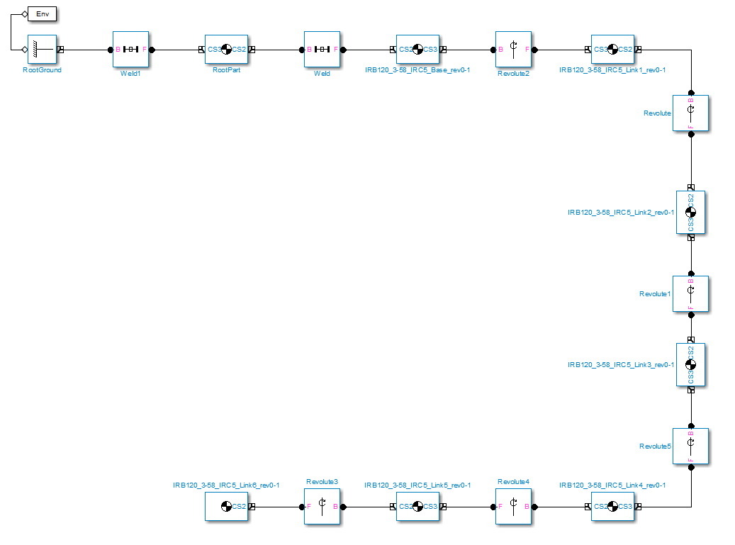
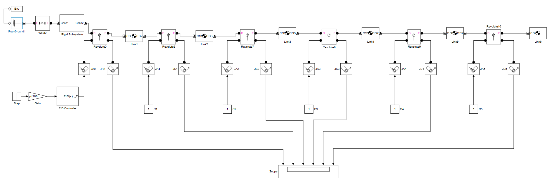
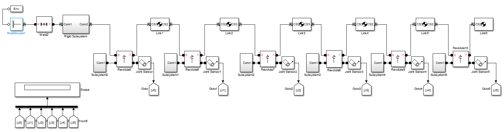
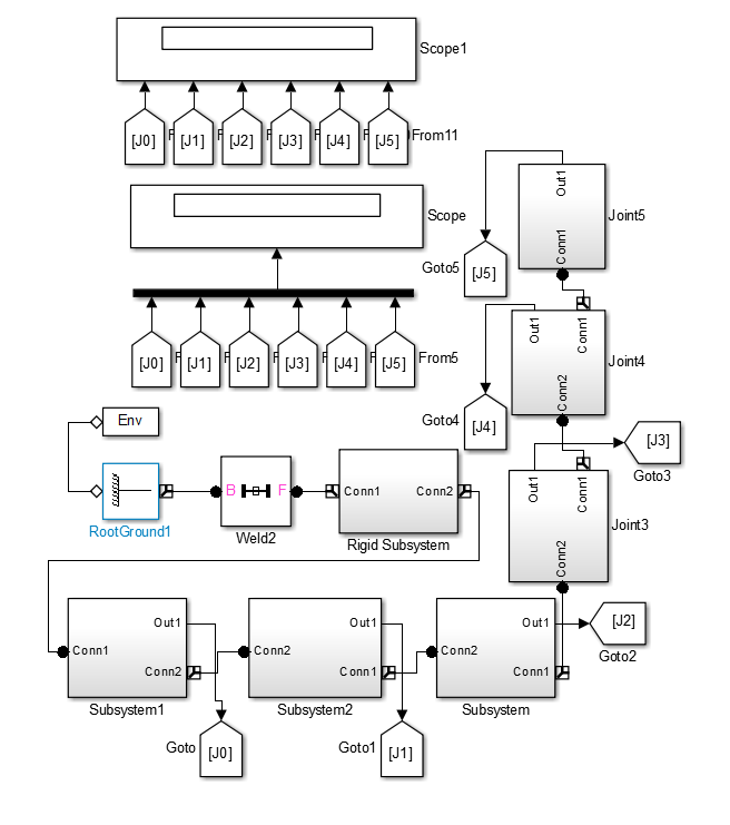
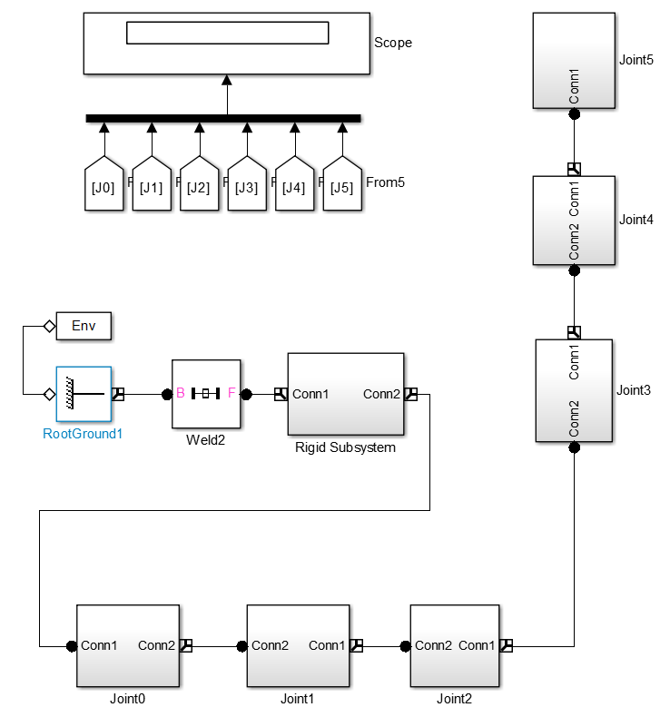
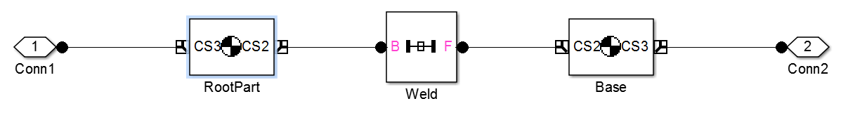
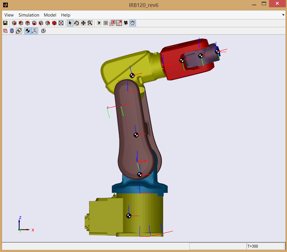
The CAD model was obtained from ABB's official file repository and imported into Simulink's SimMechanics toolbox as STL geometry. Each link carries precise mass and inertia tensors derived from the CAD data. Coordinate frames are assigned at each joint following the DH convention.

Front view
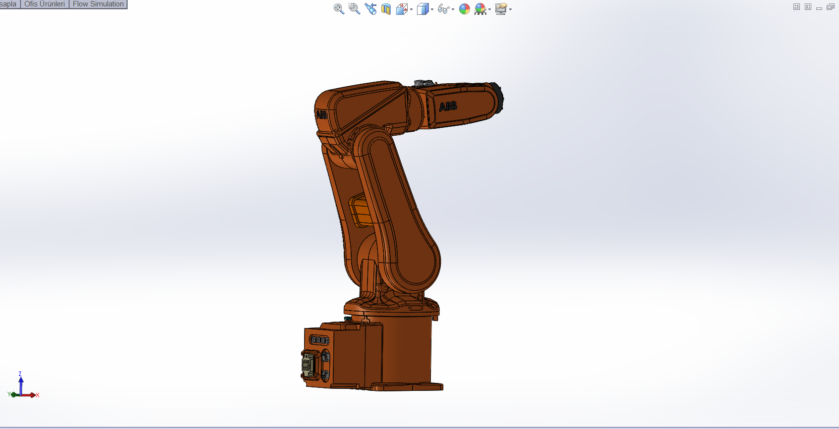
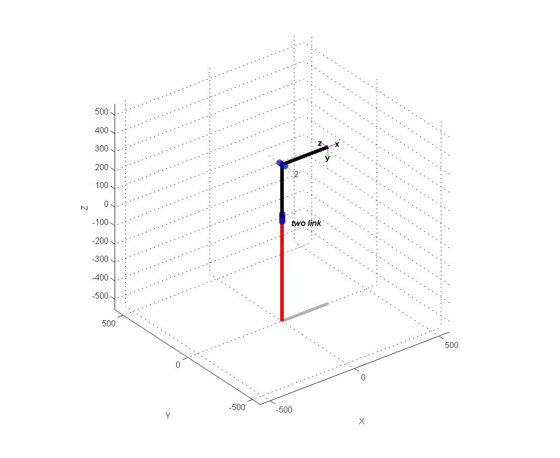
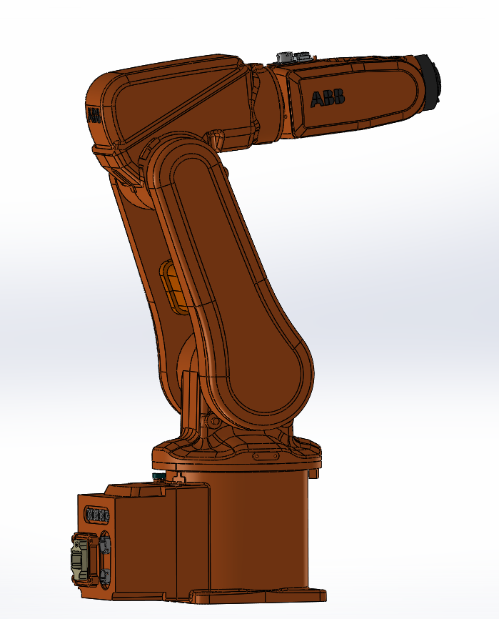
Frontal view — zero configuration
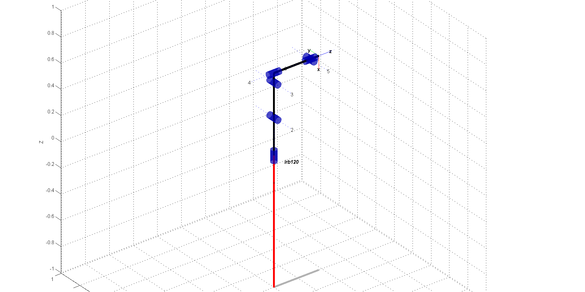
Side view
Side view
Isometric view
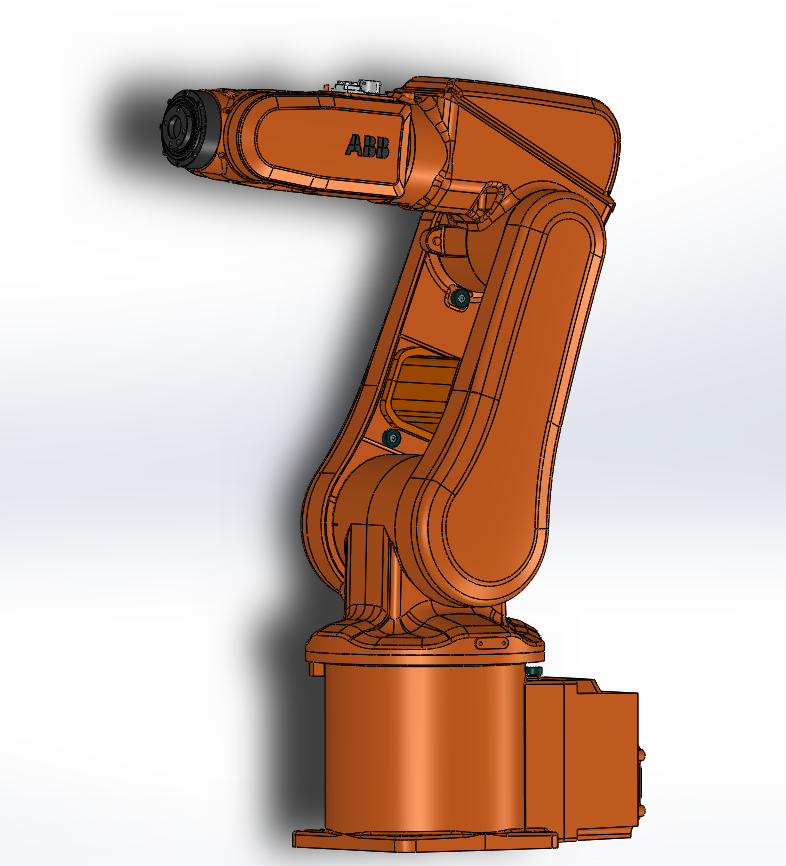
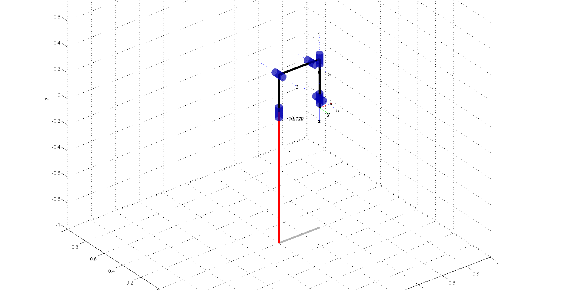
Isometric — link frames
Initial configuration
Simulation — initial configuration
04 — Kinematics

Denavit–Hartenberg parameters

The kinematic model is built using the Denavit–Hartenberg (DH) convention. A coordinate frame is attached to each joint following a four-step procedure: align the \(z\)-axis with the joint axis, define the common normal between consecutive \(z\)-axes, and express four parameters — \(d\), \(\theta\), \(a\), \(\alpha\) — that uniquely describe the transformation between adjacent frames.

Table 1 — DH parameters for the ABB IRB120
Joint \(d\) (mm) \(\theta\) (variable) \(a\) (mm) \(\alpha\) (rad) Notes
1 — Rotation (base) 290 \(\theta_1\) 0 \(-\pi/2\) Base height 290 mm
2 — Lower arm 0 \(\theta_2 - \pi/2\) 270 \(0\) Upper arm link 270 mm
3 — Elbow 0 \(\theta_3\) 70 \(-\pi/2\) Forearm offset 70 mm
4 — Wrist roll 302 \(\theta_4\) 0 \(+\pi/2\) Wrist length 302 mm
5 — Wrist pitch 0 \(\theta_5\) 0 \(-\pi/2\)
6 — Tool flange 72 \(\theta_6 + \pi\) 0 \(0\) Flange offset 72 mm

The total kinematic chain length is \(290 + 270 + 70 + 302 + 72 = 1004\) mm along the fully-extended configuration. The nominal rated reach of the IRB120 is 580 mm due to joint-limit constraints and workspace geometry.

05 — Forward Kinematics

Homogeneous transformation matrices

Forward kinematics answers: given a set of joint angles, where is the end-effector? Using DH parameters, each consecutive frame transformation is a 4×4 homogeneous transformation matrix. Multiplying them in sequence yields the full pose of the tool frame in the base frame.

DH transformation — frame i−1 to frame i
$$T_{i}^{i-1} = \begin{bmatrix} \cos\theta_i & -\sin\theta_i\cos\alpha_i & \sin\theta_i\sin\alpha_i & a_i\cos\theta_i \\ \sin\theta_i & \cos\theta_i\cos\alpha_i & -\cos\theta_i\sin\alpha_i & a_i\sin\theta_i \\ 0 & \sin\alpha_i & \cos\alpha_i & d_i \\ 0 & 0 & 0 & 1 \end{bmatrix}$$
End-effector pose — base frame to tool frame
$$T_6^0 = T_1^0 \cdot T_2^1 \cdot T_3^2 \cdot T_4^3 \cdot T_5^4 \cdot T_6^5 = \begin{bmatrix} R_{3\times3} & \mathbf{p}_{3\times1} \\ \mathbf{0}_{1\times3} & 1 \end{bmatrix}$$

The upper-left 3×3 block \(R\) encodes the orientation of the tool frame (roll–pitch–yaw). The vector \(\mathbf{p} = [x,\, y,\, z]^\top\) gives the Cartesian position of the tool origin in the base frame.

06 — Inverse Kinematics

Joint angle computation

Inverse kinematics solves the inverse problem: given a desired end-effector position and orientation, compute the joint angles that achieve it. For a 6-DOF manipulator this is a system of 6 non-linear equations in 6 unknowns.

A geometric decoupling approach is applied. Because joints 4–6 form a spherical wrist — all three axes intersect at a single point — the position subproblem (joints 1–3) and the orientation subproblem (joints 4–6) can be solved independently.

1
Wrist centre computation
Back-calculate the wrist centre position \(\mathbf{p}_{wc}\) from the desired tool pose and the known offset \(d_6\).
2
Solve joints 1–3 (position)
\(\theta_1\) from the XY projection of \(\mathbf{p}_{wc}\). \(\theta_2, \theta_3\) resolved geometrically from the triangle formed by \(a_2\), \(a_3\), \(d_4\).
3
Solve joints 4–6 (orientation)
With \(R_0^3\) known, compute the wrist rotation \(R_3^6 = (R_0^3)^\top R_0^6\). Extract \(\theta_4, \theta_5, \theta_6\) as ZYZ Euler angles.
4
Configuration selection
Multiple solution branches exist (elbow-up / elbow-down). The branch closest to the current joint state is selected to minimise motion.
07 — Velocity Kinematics

Jacobian matrix

The Jacobian \(J\) maps joint velocities \(\dot{\mathbf{q}}\) to end-effector linear and angular velocities. For a 6-DOF arm, \(J \in \mathbb{R}^{6 \times 6}\) is partitioned into a linear part \(J_v\) and an angular part \(J_\omega\):

Velocity relationship
$$\begin{bmatrix} \mathbf{v} \\ \boldsymbol{\omega} \end{bmatrix} = J(\mathbf{q})\,\dot{\mathbf{q}}, \qquad J = \begin{bmatrix} J_v \\ J_\omega \end{bmatrix} \in \mathbb{R}^{6 \times 6}$$ $$J_i = \begin{bmatrix} \mathbf{z}_{i-1} \times (\mathbf{p}_n - \mathbf{p}_{i-1}) \\[4pt] \mathbf{z}_{i-1} \end{bmatrix} \quad \text{(column } i \text{ for revolute joint } i\text{)}$$

Singularities occur when \(\det(J) = 0\): the arm loses one or more degrees of freedom. For the IRB120, singularities arise at fully-extended configurations (shoulder singularity) and when joints 4 and 6 align (wrist singularity). Trajectory planning avoids these regions.

08 — Robot Dynamics

Lagrangian formulation

The dynamic model predicts the joint torques required to produce a given motion, accounting for inertia, Coriolis and centrifugal effects, and gravity. The Euler–Lagrange method starts from the kinetic and potential energies of all links.

Lagrangian and energy terms
$$\mathcal{L} = K - P \qquad \text{(kinetic minus potential energy)}$$ $$K = \frac{1}{2} \sum_{i=1}^{6} \left[ m_i\,\dot{\mathbf{v}}_i^\top\dot{\mathbf{v}}_i + \boldsymbol{\omega}_i^\top \mathbf{I}_i \boldsymbol{\omega}_i \right]$$ $$P = \sum_{i=1}^{6} m_i\, g\, z_{c_i}$$
Euler–Lagrange equation (one per joint)
$$\tau_i = \frac{d}{dt}\!\left(\frac{\partial \mathcal{L}}{\partial \dot{q}_i}\right) - \frac{\partial \mathcal{L}}{\partial q_i}$$
Robot dynamics — matrix form
$$\boldsymbol{\tau} = M(\mathbf{q})\,\ddot{\mathbf{q}} + C(\mathbf{q},\dot{\mathbf{q}})\,\dot{\mathbf{q}} + G(\mathbf{q})$$
Inertia matrix
\(M(\mathbf{q}) \in \mathbb{R}^{6\times6}\)
Positive definite; configuration-dependent
Coriolis / centrifugal
\(C(\mathbf{q},\dot{\mathbf{q}}) \in \mathbb{R}^{6\times6}\)
Velocity-dependent coupling terms
Gravity vector
\(G(\mathbf{q}) \in \mathbb{R}^{6}\)
Configuration-dependent static loads

For each joint, the partial derivatives of the Lagrangian were evaluated symbolically with respect to DH-derived expressions for link velocities and positions. The resulting torque equations were implemented as Simulink function blocks and verified against SimMechanics computed joint reaction forces.

09 — Trajectory Generation

Smooth joint-space planning

A quintic polynomial generates smooth reference trajectories for each joint. The polynomial satisfies six boundary conditions — initial and final position, velocity, and acceleration — ensuring the robot starts and ends at rest with zero acceleration.

For painting tasks, smooth trajectories are essential: abrupt velocity changes cause brush-pressure variations that degrade stroke quality. The quintic ensures zero jerk at waypoints when connecting multiple segments.

Quintic polynomial trajectory
$$q(t) = a_0 + a_1 t + a_2 t^2 + a_3 t^3 + a_4 t^4 + a_5 t^5$$
Six boundary conditions
$$q(0) = q_0,\quad q(t_f) = q_f$$ $$\dot{q}(0) = 0,\quad \dot{q}(t_f) = 0$$ $$\ddot{q}(0) = 0,\quad \ddot{q}(t_f) = 0$$
10 — Implementation

Simulink control architecture

The closed-loop control system is implemented entirely in Simulink. A six-channel PID controller — one per joint — receives the quintic trajectory reference and drives the SimMechanics mechanical model. Joint angle sensors provide position feedback to close each loop.

Top-level Simulink model
Top-level model — trajectory reference, PID bank, SimMechanics plant
Joint control subsystem
Rigid body block
Rigid body link block
PID controller
PID controller — P, I, D gains
Simulink model 5
Trajectory generator block
Simulink model 6
Forward kinematics output
Simulink model 7
Dynamic torque computation subsystem
Simulink model 8
Scope configuration
11 — Results

3D simulation & scope outputs

The simulation runs the full trajectory sequence: the robot moves from an initial configuration through the planned waypoints, with SimMechanics rendering the 3D motion in real time. Scope blocks capture joint angles, velocities, and control torques for all six axes throughout the motion.

Final configuration
Simulation — final configuration after trajectory
Joint angle trajectories
Joint angle tracking — all 6 axes
Position tracking
End-effector position tracking
Scope output 3
Velocity profiles
Scope output 4
Torque demands — joints 1–3
Scope output 5
Torque demands — joints 4–6
Matlab scope
Matlab scope — composite output
12 — Model Parameters

Full simulation specification

Robot model
ABB IRB120 3/0.6
Compact articulated arm
Degrees of freedom
6
All revolute (RRRRRR)
Simulation solver
ode45
Runge–Kutta 4/5, variable step
Relative tolerance
1 × 10⁻³
Integration accuracy
Joint control
PID
Independent per axis
Trajectory type
Quintic
5th-order polynomial, joint space
Dynamics model
Lagrangian
\(M\ddot{q} + C\dot{q} + G\) formulation
Geometry source
ABB STL files
Official CAD from ABB repository
Environment
Matlab R2014a
Simulink + SimMechanics toolbox
Base height \(d_1\)
290 mm
Upper arm \(a_2\)
270 mm
Wrist length \(d_4\)
302 mm